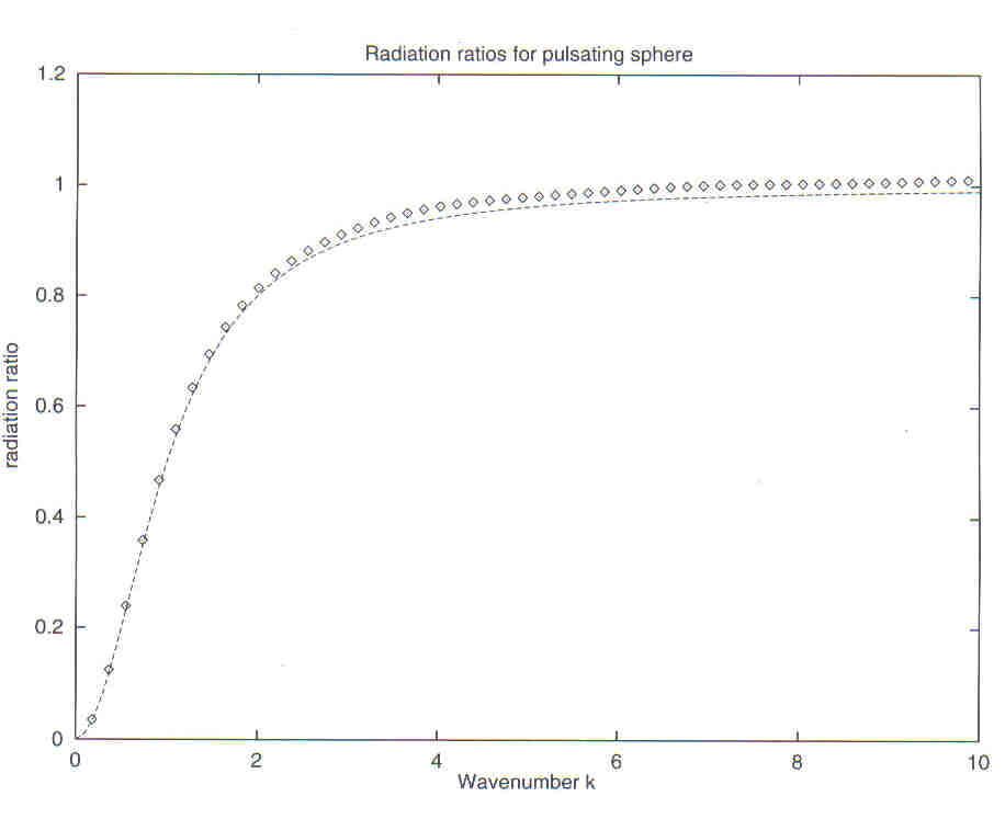
Fig 5.2. Radiation ratio curve for pulsating sphere (- exact, ą computed).
The acoustic medium is air at 20 celcius and 1 atmosphere so the speed of sound is 344m/s. The chosen frequency of the test is 400Hz, hence k = 7.31. For the first two tests, the velocity potential defined by f(p) = i/4H0(kr), with r being the distance from the point p to the centre of the square, is clearly a solution of the Helmholtz equation in the exterior domain. The boundary velocity is given by differentiation this expression for f(p) with respect to the normal to the boundary at p for each collocation point p on S.
In the first two tests the Dirichlet and Neumann boundary conditions arising from this potential is processed by AEBEM2. The solution is given at the points (0,0.15), (0.05,0.15), (0.1,0.15) and (0.05,-0.1). Comparisons between the exact and numerical solutions are given in Table 5.A.
Table 5.A: Results from AEBEM2_T
| point | exact solution | numerical solution | numerical solution
| | to Dirichlet condition | to Neumann condition
| (0.000,0.150) |
0.0176 + i 0.2100 | 0.0198 + i 0.2079 | 0.0181 + i 0.2104
| (0.050,0.150) |
0.0394 + i 0.2177 | 0.0415 + i 0.2154 | 0.0397 + i 0.2181
| (0.100,0.150) |
0.0176 + i 0.2100 | 0.0198 + i 0.2079 | 0.0181 + i 0.2104
| (0.050,-0.100) |
-0.0398+ i 0.1804 | -0.0375 + i 0.1792 | -0.0396 + i 0.1808 | | ||||
The acoustic medium is air at 20 celcius and 1 atmosphere so that the speed of sound is c = 344m/s. In the first two test problems the acoustic field in the exterior is defined to be
|
Table 5.B: Results from AEBEM3_T
| point | exact solution | numerical solution | numerical solution
| | to Dirichlet condition | to Neumann condition
| (0,0,2) |
-0.4360 - i 0.2447 | -0.4628 - i 0.1897 | -0.5011 - i 0.2389
| (0,0,4) |
0.1302 + i 0.2133 | 0.1557 + i 0.1960 | 0.1614 + i 0.2274
| (0,0,8) |
-0.0572 + i 0.1112 | -0.0431 + i 0.1175 | -0.0549+ i 0.1284
| (0,0,-2) |
-0.4360 - i 0.2447 | -0.4628 - i 0.1897 | -0.5011 - i 0.2389 | | ||||
In this example a comparison of the computed and exact sound pressures are given. The magnitudes (in decibels) and the phases (in degrees) are given in Table 5.C. The values are computed from the sound pressures in line with the methods described in Section 1.3.
Table 5.C: Results from IBEM3_T
| point | exact solution | numerical solution | numerical solution
| | to Dirichlet condition | to Neumann condition
| (0,0,2) |
72.8dB, -60.7° | 72.8dB, -69.8° | 73.2dB, -64.7°
| (0,0,4) |
69.8dB, 148.6° | 69.8dB, 139.5° | 70.2dB, 144.4°
| (0,0,8) |
66.8dB, -152.8° | 66.8dB, -161.9° | 67.2dB, -157.1°
| (0,0,-2) |
72.8dB, -60.7° | 72.8dB, -69.8° | 73.2dB, -64.7° | | ||||
The program AEBEMA_T also shows results from a sphere scattering a point source where in the first case the potential on the sphere is assigned the incident potential in a Dirichlet condition, so that the sphere is effectively invisible. In the second case the sphere represents a rigid (non-vibrating) acoustically hard scatterer. An application similar to these examples is given in the next Section.
In each test problem the frequency ranges from 10 Hz to 1000Hz in 10 Hz steps. The purpose of the first test problem is to plot the radiation ratio of a pulsating sphere. In the test problem the surface velocity is prescribed the value of unity on each element. Note that the radiation ratio refers to the shape of the boundary condition, the amplitude is arbitrary. The results from the test are directed to the file AEBEMA.OUT. The exact radiation ratio for a sphere of radius unity, pulsating at wavenumber k is [(k2)/( k2+1)]. A comparison of the computed and exact radiation ratios are given in Figure 5.2.
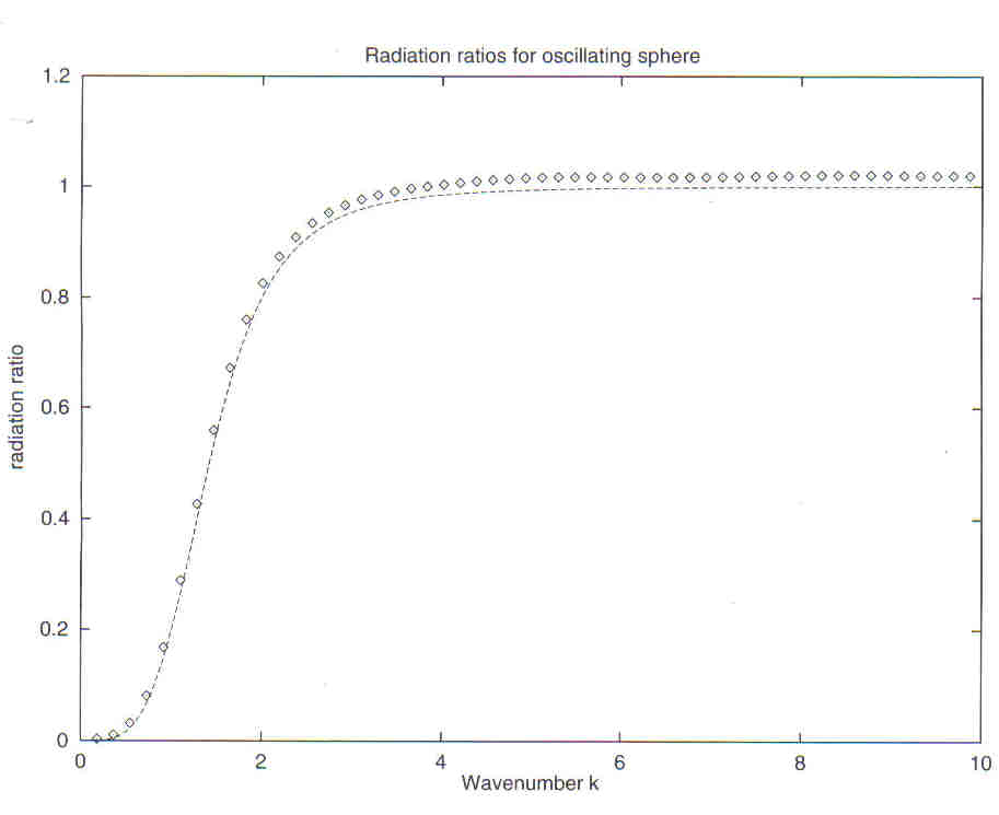
Results for an oscillating sphere, that is the sphere vibrating up
and down without changing volume, are given in Figure 5.3.
These results can be obtained from a test problem similar to
AEBEMA by setting the same Neumann surface condition but with
SFVAL(ITEST,ISP)=SELCNT(ISP,2). The exact radiation ratio of an oscillating sphere is [(k4)/( 4+k4)].