5.7 Application: Engine Noise Analysis
A computational prediction of the acoustic properties of an engine
design can be useful. It
enables the engineer to analyse the noise output of an
engine at the early design stage and hence make the necessary
adjustments.
This Section is on the prediction of the noise output from
an engine block. In order to do this the engine
is modelled as an arbitrary three-dimensional vibrating surface
radiating into free-space.
From the theoretical point of view, the
BEM can closely represent the the physical situation of the
engine in free-space or in an anechoic chamber.
In order to apply the method, the surface of the block must
be simplified so some of the surface details need to be omitted.
The boundary element method in this application has been considered
by a number of researchers, for example references [52],
[76].
For this type of problem subroutine
AEBEM3 is most suitable. However, the results
presented in this Section were obtained using a prototype
program that uses similar elements and method
but preceded AEBEM3 by a number of years. The
work of this Section was originally published in
reference [45]
and the reader is advised to consult that paper if further
details are required.
The velocity distribution (at each frequency) on the surface,
required for the input of the Neumann boundary condition,
is determined through using accelerometers fitted at
a set number of points over the surface.
In order to apply the boundary element method the
surface is simplified and represented by around 550 planar triangular
elements with the vertices of the
triangles generally being at the accelerometer points.
On each boundary element the surface velocity is determined
by averaging the values of the surface velocity at the three
vertices. At vertices where there was no accelerometer
reading the velocity was prescribed a zero value. The BEM mesh for the engine block
is shown in figure 5.4.
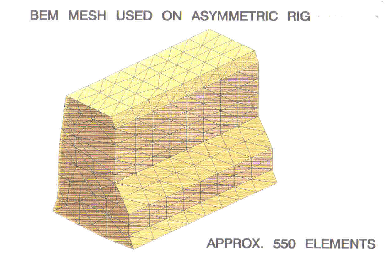
Fig 5.4. The BEM mesh of the engine block.
The sound power was computed at a range of frequencies
from 400Hz to 2400Hz. The results of this are
compared with measured results
in Figure 5.5. The measured results
are found by integrating the readings from a microphone array;
a method based on
equation (1.12).
The boundary element mesh of the rig, showing the computed
surface intensity pattern at 1120Hz, is shown on the cover
of this textbook. The colours range from deep blue on the
areas of low intensity through green, yellow, orange red and
to purple on the areas of high intensity. Only the
middle-left cylinder was excited in the test and this is
reflected in the results.
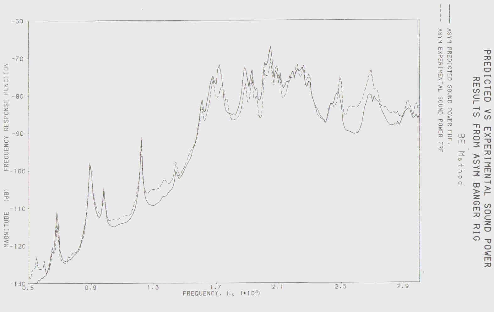
Fig 5.5. Comparison betwen computed and measured sound powers.
Return to boundary-element-method.com/acoustics
Return to boundary-element-method.com