6.6 Application: Loudspeaker Enclosure
In this Section a modal analysis of the air-tight interior of
a test axially symmetric loudspeaker is carried
out via the boundary element method using subroutine AMBEMA.
Some of the results are compared with results from physical experiment.
For further details on this application and the results obtained
the reader is referred to [48].
6.6.1 Background
The effect of the fluid-loading of the air on the cone is
of some interest to loudspeaker designers.
The coupling of air external to the loudspeaker to the motion of
the cone is considered experimentally in Jones [35], wherein
the difference between the forced vibration of a cone in air and its
vibration in a vacuum is found to be negligible. However, it is
expected that the presence of the air inside the cabinet can have
a significant effect on the vibration of the cone
due to the relatively small, enclosed volume occupied by the air.
The greatest effect of air loading on the vibration of the cone occurs
when there are large changes in pressure over the surface of the
cone. The maximum change in pressure will be at acoustic resonant
frequencies and therefore the corresponding mode shapes are studied.
By applying the methods to an axisymmetric loudspeaker, the acoustic
properties may be examined
whilst reducing the dimension of the problem by one and thus
reducing the computational expense when compared to the full three-dimensional
analysis that is necessary for a general loudspeaker design.
In addition, considerable previous work has been done on the
structural vibration of axially symmetric loudspeaker drive units
(see Jones [35] and Jones and Henwood [36], for example).
In this work we show results for the cabinet shown in Figure 6.1,
which is basically a cylinder 120mm deep and 132mm in diameter. The loudspeaker
has a conical drive unit of radius 80mm fitted.
Given these dimensions, the lowest cabinet resonance occurs around
1kHz, and the cabinet resonances can be observed in sound
pressure measurements outside the cabinet.
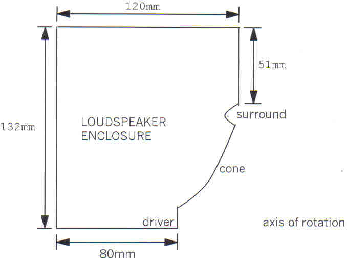
Fig. 6.1. Diagram of the axisymmetric cabinet.
6.6.2 Particular implementations of computational method and
Measurements
For the application of the boundary element method the boundary
of the generator of the loudspeaker is approximated
by 32 conical elements of approximately equal length along the generator,
as shown in Figure 6.1.
Solutions were sought in the k-ranges [0.0,5.0], [5.0,10.0], [10.0,15.0]
and so on. In each range quadratic interpolation was
applied ( NK=3). The approximations to the mode shapes are then obtained
at around 100 points in the interior.
For the measurement of the resonant frequencies,
microphone readings of the sound pressure
were taken at various positions within the cabinet.
Measurements were made through all frequencies of interest, commencing
at 20Hz and going through to 20kHz. The peaks in the response
inform us of the internal resonant frequencies.
Firstly the five lowest resonant frequencies obtained through the
boundary element methods and the results
obtained by measurement are compared in Table 6.B.
|
Table 6.B: Computed and measured loudspeaker resonant frequencies
| Mode | Boundary Element | Experimental
| 1 | 1414 Hz | 1318 Hz
| 2 | 1590 Hz | 1679 Hz
| 3 | 2232 Hz | 2133 Hz
| 4 | 2815 Hz | 2691 Hz
| 5 | 2876 Hz | 3306 Hz | | | | | | |
The major contribution to the discrepancy between the measured and
calculated values is believed to be the simplicity of the model
chosen, which fails to include any internal structure to the
loudspeaker. In addition, the maximum pressure occurs at slightly
different frequencies for different microphone positions.
Figure 6.2 shows the first, third and fifth mode shapes obtained via the boundary element method.
The mode shapes are constructed from the returned values of
f* in the domain. The values on the contours are arbitrary.
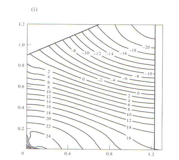
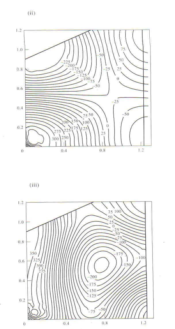
Fig 6.2. The first, third and fifth mode shape of the loudspeaker cabinet.
Return to boundary-element-method.com/acoustics
Return to boundary-element-method.com