6.6 Application: Loudspeaker Enclosure

In this Section a modal analysis of the air-tight interior of a test axially symmetric loudspeaker is carried out via the boundary element method using subroutine HMBEMA. Some of the results are compared with results from physical experiment. For further details on this application and the results obtained the reader is referred to [48].

6.6.1 Background

The effect of the fluid-loading of the air on the cone is of some interest to loudspeaker designers. The coupling of air external to the loudspeaker to the motion of the cone is considered experimentally in Jones [35], wherein the difference between the forced vibration of a cone in air and its vibration in a vacuum is found to be negligible. However, it is expected that the presence of the air inside the cabinet can have a significant effect on the vibration of the cone due to the relatively small, enclosed volume occupied by the air.

The greatest effect of air loading on the vibration of the cone occurs when there are large changes in pressure over the surface of the cone. The maximum change in pressure will be at Helmholtz resonant frequencies and therefore the corresponding mode shapes are studied. By applying the methods to an axisymmetric loudspeaker, the Helmholtz properties may be examined whilst reducing the dimension of the problem by one and thus reducing the computational expense when compared to the full three-dimensional analysis that is necessary for a general loudspeaker design. In addition, considerable previous work has been done on the structural vibration of axially symmetric loudspeaker drive units (see Jones [35] and Jones and Henwood [36], for example). In this work we show results for the cabinet shown in Figure 6.1, which is basically a cylinder 120mm deep and 132mm in diameter. The loudspeaker has a conical drive unit of radius 80mm fitted. Given these dimensions, the lowest cabinet resonance occurs around 1kHz, and the cabinet resonances can be observed in sound pressure measurements outside the cabinet.

Fig. 6.1. Diagram of the axisymmetric cabinet.

6.6.2 Particular implementations of computational method and Measurements

For the application of the boundary element method the boundary of the generator of the loudspeaker is approximated by 32 conical elements of approximately equal length along the generator, as shown in Figure 6.1. Solutions were sought in the k-ranges [0.0,5.0], [5.0,10.0], [10.0,15.0] and so on. In each range quadratic interpolation was applied ( NK=3). The approximations to the mode shapes are then obtained at around 100 points in the interior.

For the measurement of the resonant frequencies, microphone readings of the sound pressure were taken at various positions within the cabinet. Measurements were made through all frequencies of interest, commencing at 20Hz and going through to 20kHz. The peaks in the response inform us of the internal resonant frequencies.

6.6.3 Results

Firstly the five lowest resonant frequencies obtained through the boundary element methods and the results obtained by measurement are compared in Table 6.B.


Table 6.B: Computed and measured loudspeaker resonant frequencies
Mode	Boundary Element	Experimental
1	1414 Hz	1318 Hz
2	1590 Hz	1679 Hz
3	2232 Hz	2133 Hz
4	2815 Hz	2691 Hz
5	2876 Hz	3306 Hz

The major contribution to the discrepancy between the measured and calculated values is believed to be the simplicity of the model chosen, which fails to include any internal structure to the loudspeaker. In addition, the maximum pressure occurs at slightly different frequencies for different microphone positions.

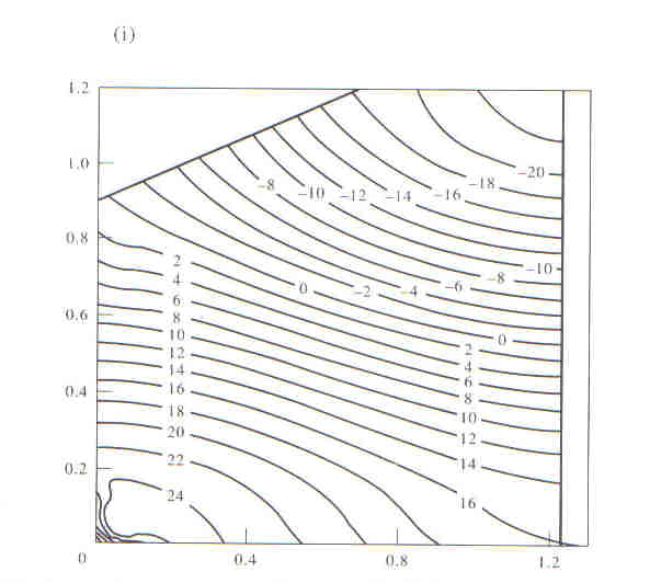
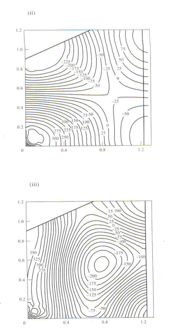
Figure 6.2 shows the first, third and fifth mode shapes obtained via the boundary element method. The mode shapes are constructed from the returned values of f^* in the domain. The values on the contours are arbitrary.

Fig 6.2. The first, third and fifth mode shape of the loudspeaker cabinet.

Return to boundary-element-method.com/helmholtz
Return to boundary-element-method.com